
Chips’nCode has always been a bit mixed because my own background is mixed. Before I moved into secondary teaching, I came out of biology, molecular biology and ecology. These days I teach general science, Biology and Psychology at secondary level, alongside Digital Technologies and Mathematics. I am also a radio amateur, VK4MPB/VK7MPB, so radio, electronics and computing tend to turn up in the same places eventually.
A radiosonde is a good example of why I like the overlap. It is simultaneously a set of environmental sensors, a radio transmitter, a stream of digital data and a moving point in three-dimensional space. A weather satellite brings in orbital motion, waves, Doppler shift, antennas, digital signals and image data. Even an ordinary FM station gives you a useful way to make frequency, bandwidth, signal strength and noise visible.
Over the past year I have been building more of that thinking into the Year 9 Digital Technologies class I teach. We have worked with Python, networks, packets, addresses, DNS, routers, latency, bandwidth and the physical systems underneath the internet. This is not much of a curriculum detour. The Australian Curriculum: Digital Technologies explicitly covers digital systems and networks, including how data is transmitted, managed and secured. The wireless part is often the bit students are asked to accept without ever seeing it.
An RTL-SDR gives us a way to look at that radio layer directly. It is a small USB software-defined receiver. Add an antenna and a computer and you can examine a large part of the radio spectrum around you. The spectrum is a live graph of signal strength across a range of frequencies. The waterfall is that same graph recorded down the screen over time. Signals become visible shapes: you can see how wide they are, watch them come and go, compare their strength, record them and, when they contain digital information, hand them to software that can decode what is being transmitted.
You can do all of that without transmitting anything and without needing an amateur radio licence.
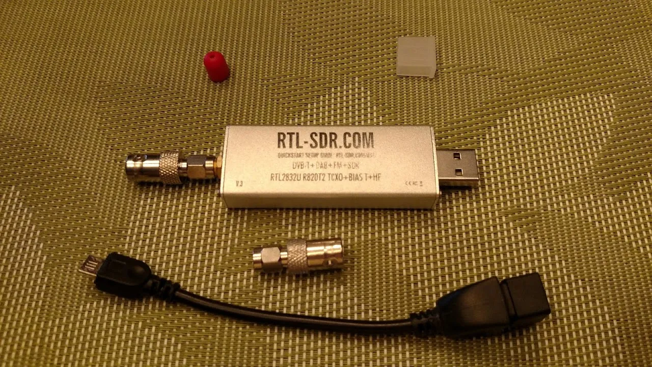
An RTL-SDR Blog V3 receiver with the adapters supplied in the multipurpose kit. Photo: Joeceads, Wikimedia Commons, CC BY-SA 4.0.
Getting an RTL-SDR
There are a lot of cheap USB digital-television dongles, usually labelled DVB-T, being sold as RTL-SDRs. Some are perfectly usable, but for a first receiver I would buy the genuine RTL-SDR Blog V3 dongle with the multipurpose dipole kit. It gives you a stable receiver, a threaded SMA antenna socket and an antenna set that can be rearranged for broadcast FM, amateur repeaters, aircraft and satellites.
For Australian buyers, OpenSourceSDRLab’s RTL-SDR Blog V3 kit listing is usually worth checking before the larger marketplaces. Their product naming has changed over time, so I would check the current dongle revision and kit contents on the listing rather than relying on an old screenshot.
I have no interest in making this a shopping guide. The important bits are an RTL2832U-based receiver, a stable internal frequency reference, an SMA connector and an antenna you can put somewhere sensible. If you already own a working RTL-SDR, use it.
Getting the antenna right
The older RTL-SDR kits often came with a single magnetic-base telescopic whip. A whip still works, especially for strong local signals, and it is a perfectly good way to start. The current RTL-SDR Blog kit is more useful because the same hardware can also be assembled as a dipole.
The kit has a centre-fed dipole base, two long telescopic elements that extend from roughly 23 cm to 1 m, two short elements that cover about 5 cm to 13 cm, a coaxial-cable extension, tripod and suction mount. The RTL-SDR Blog dipole guide is worth keeping open the first few times you use it.
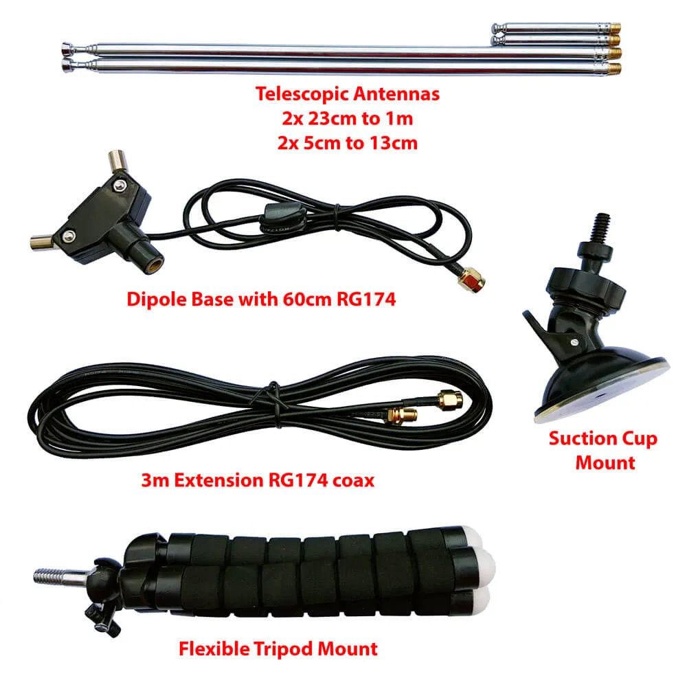
The dipole kit components: long and short telescopic elements, centre-fed base, coax extension, suction mount and flexible tripod. Image: RTL-SDR Blog.
A dipole is simply two conductive elements fed in the middle. The wavelength tells you how long one complete radio wave is. A basic half-wave dipole is half a wavelength from end to end, so each of its two elements is approximately one quarter of a wavelength.
- λ
- wavelength, in metres
- c
- speed of light, about 300,000,000 metres per second
- f
- frequency, in hertz
At 145 MHz, for example, a full wavelength is about 2.07 metres, so each dipole element is about 51 cm. Around 137 MHz for weather satellites, each element is about 54 cm. At 1090 MHz for ADS-B, a quarter wavelength is only about 6.9 cm. For receive-only work these are useful starting lengths rather than dimensions that need to be exact to the nearest millimetre.
For most terrestrial signals in the VHF and UHF ranges, meaning very high frequency and ultra high frequency, set the dipole vertically. If you only have a whip, a vertical whip is also a sensible default. For 137 MHz weather satellites, the same dipole can be laid horizontally and opened into a V. RTL-SDR Blog recommends about 53.4 cm per element and an included angle of roughly 120 degrees.
The supplied kit is intended for receiving. Do not connect it to a transmitter.
Try itTurn the kit into a 2 m dipole
Keep the feed point near the middle and arrange the two elements vertically, one above the other. For receive-only experimenting, getting both elements close to the correct length is enough to start.
Pick your receiver software
The job is the same on every desktop platform: talk to the RTL-SDR, show the spectrum and waterfall, choose the reception mode, set the width of the slice you want to receive, and adjust the receiver’s sensitivity. Radio software calls those last three controls the mode, filter width and gain.
Receiver software by platform
SDR++ is available across the main desktop platforms. Gqrx and other receivers use the same basic settings: frequency, mode, filter width and gain.
On Android, SDR++ can work with supported USB SDR hardware over OTG. Direct RTL-SDR use on iPhone and iPad is much less convenient, so I use iOS mainly for pass prediction and tracking rather than as the receiver itself.
Use the program written for the signal you want to decode. SatDump handles satellite telemetry and imagery. radiosonde_auto_rx handles weather balloons. ADS-B has its own decoders. GNU Radio becomes useful once there is some value in seeing how the receiver itself is put together.
Start with ordinary FM radio
The first thing I would receive is an ordinary FM broadcast station. It is not particularly exotic, which is exactly why it is useful. In Australia the broadcast FM band runs from 87.5 to 108 MHz, and a strong local station gives you a signal you already know should work.
Use the dipole vertically with both long elements somewhere around 70–80 cm, or use a vertical whip. Tune a station you know, select WFM, meaning wideband FM, and get clean audio. Then deliberately change one thing at a time while watching the spectrum and listening to the result.
Try itReceive a local FM station
Start with the station centred in the filter. Once it sounds clean, narrow the filter, tune slightly high or low, reduce the RF gain, increase it again and change the antenna length. RF gain controls how strongly the receiver amplifies incoming radio signals. Watch the waterfall as you make each change.
Success is not just hearing the station. You should be able to make the audio worse on purpose and explain why.
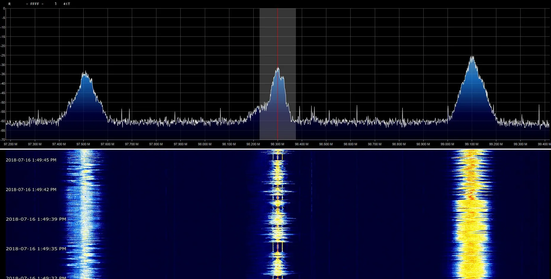
An SDR waterfall in the FM broadcast band. Speech and music leave different patterns down the waterfall even when the station stays on the same channel. Image: Wtshymanski, Wikimedia Commons, CC BY-SA 4.0.
Listen to amateur radio
Amateur radio is a licensed service for people who want to communicate, experiment and learn about radio. That can mean ordinary voice conversations, digital messages, satellite contacts, long-distance shortwave work, emergency communications, antenna building or simply seeing how far a small amount of power will travel. It is a broad hobby because radio itself is broad. You need the appropriate qualification and callsign before transmitting, but anyone can listen. An RTL-SDR therefore gives you a useful way to explore the amateur bands and hear how they are used before deciding whether you want to get on air yourself.
For a first amateur-radio listening exercise with an RTL-SDR in Australia, start with the 2 metre band, 144–148 MHz, and the 70 centimetre band, 430–450 MHz. These names refer roughly to the wavelength, not the size of the antenna. The Wireless Institute of Australia (WIA) publishes Australia-specific band plans showing how those allocations are divided between voice, repeaters, satellites, data and other uses.
An amateur repeater receives a signal on one frequency and retransmits it on another, often from a high site that covers a wide area. It may sit quiet for a while and then suddenly come alive. On the waterfall you will see the narrow FM signal appear, hear the conversation, then watch it disappear when the operator stops transmitting. You may also hear the repeater identify itself.
Rather than dragging the tuning control around and hoping somebody happens to speak, Australian readers can use the WIA Repeater Directory to find an operational analogue FM repeater nearby. Outside Australia, or as a second source within it, RepeaterBook provides an international repeater directory with an Australian listing. Use the output frequency, because that is the frequency the repeater transmits and therefore the one you want to receive.
Try itListen to a local 2 m repeater
Set the long dipole elements to about 50 cm each and mount the antenna vertically. A whip near the same length is also fine. Select NFM, meaning narrowband FM. You do not need the repeater input frequency or its CTCSS access tone, the sub-audible tone used to open some repeaters, because you are only receiving.
ADS-B: receive aircraft directly
Aircraft are a good first digital signal because there is usually something in the sky and the decoded result is immediately recognisable. ADS-B stands for Automatic Dependent Surveillance–Broadcast. Aircraft use it to broadcast information such as identity, position, altitude and speed. Most Mode S and ADS-B traffic you will receive with this setup uses 1090 MHz.
Start in SDR++ rather than going straight to a decoder. Put the receiver on 1090 MHz and watch. You are not looking for a continuous tone or a voice signal. ADS-B consists of very short pulse bursts, so with aircraft in range you should see repeated flashes on the waterfall.
The short elements in the RTL-SDR kit are the right ones here. A theoretical quarter wavelength at 1090 MHz is about 6.9 cm, which sits comfortably inside their adjustment range.
Once you have seen the activity, hand the dongle to an ADS-B decoder. On Windows, Dump1090 for Windows can receive directly from an RTL-SDR and includes a local web map. On Linux and Raspberry Pi, dump1090/readsb-based installations are common, and a small Pi can become a permanent receiver that serves its aircraft map over your network. The original dump1090 source is also useful if you want to see how the decoder works.
Try itSee 1090 MHz traffic before decoding it
Keep the antenna vertical and somewhere reasonably clear of the computer. At this stage the exact demodulation mode is not important because you are using the spectrum display rather than listening to audio.
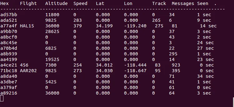
dump1090 turning locally received 1090 MHz packets into aircraft identifiers, altitudes, speeds, positions and message counts. Screenshot: RTL-SDR Blog.
Follow a radiosonde
Radiosondes are one of my favourite examples because there is quite a lot going on in a very small box. The Bureau of Meteorology and other weather services launch these instrument packages beneath balloons to sample the atmosphere. The sonde measures conditions such as temperature, humidity and pressure, obtains a position and transmits telemetry, meaning those measurements and status data, back to the ground throughout the flight.
In Australia, most of the sondes you are likely to encounter sit somewhere between 400 and 403 MHz, with 400.5, 401.5 and 402.5 MHz particularly common. Rather than scan the entire band, open the SondeHub live tracker, find an active balloon reasonably close to you and note the frequency shown for it.
Around 402 MHz, a quarter wavelength is about 18.6 cm. A vertical whip around that length is useful, or set both sides of a dipole close to that length and mount it vertically. The sonde spends much of its flight high above the ground, so a modest antenna can work surprisingly well.
Once you can see the signal, Project Horus radiosonde_auto_rx can scan, identify supported sonde types, decode their telemetry and upload positions to SondeHub. The auto_rx wiki covers installation and configuration.
Try itFind a live weather balloon
If SondeHub lists a sonde on 401.500 MHz, put 401.500 MHz into the SDR program, select narrow FM and watch for a persistent digital signal. It will look quite different from the intermittent amateur voice you heard earlier.
Open the live SondeHub map
Select a balloon to see its path, altitude, reported frequency and other flight details. If the map does not load here, open SondeHub in a new tab.
A single balloon flight gives you quite a bit to work with. The temperature, humidity and pressure are science; the packets, radio link and decoder are Digital Technologies; and the altitude, ascent rate and track give you useful mathematics. More importantly, it is real data arriving from a real instrument moving through the atmosphere, not a tidy classroom example.
Receive a weather satellite
A lot of RTL-SDR material online still begins with analogue APT, or Automatic Picture Transmission, images from NOAA-15, NOAA-18 and NOAA-19. Those satellites were retired in 2025, so the old tutorials are useful for understanding the method but no longer provide live NOAA APT targets.
The current beginner route is the digital LRPT, or Low Rate Picture Transmission, signals from the METEOR-M satellites. SatDump is the program I would use for these. It runs on Windows, macOS, Linux and Android. It can control the RTL-SDR, turn the radio signal back into digital data, and reconstruct the image.
This is also the job where the dipole kit earns its keep. Put the long elements on the base, extend each to about 53–54 cm, lay the antenna horizontally and open the elements into a broad 120-degree V. Put it outside if you can, or at least near a window and away from the computer.
The same hardware can also be opened into a V for other satellite bands. This L-band arrangement is not a 137 MHz METEOR-M antenna: its elements are shorter and it uses a reflector.
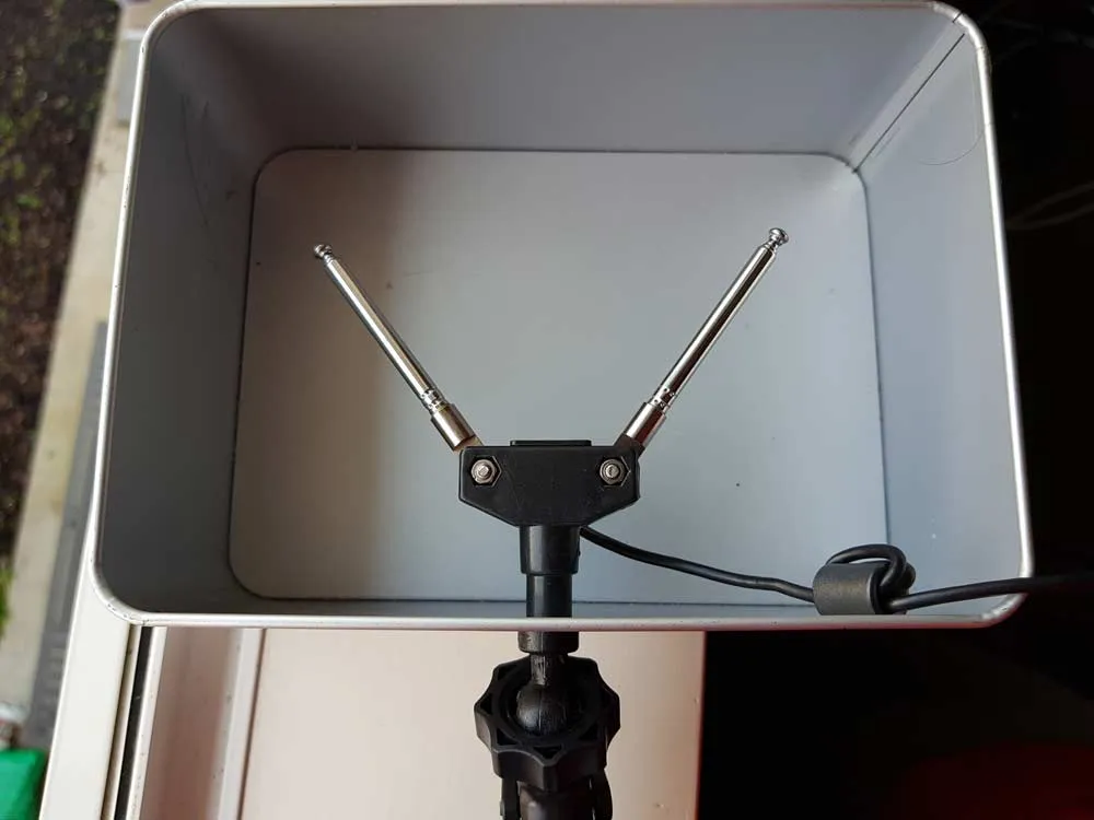
The kit arranged as a V-dipole for an L-band satellite experiment, with a metal reflector behind it. The 137 MHz setup uses longer elements and does not require the reflector. Photo: RTL-SDR Blog.
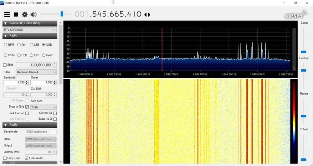
L-band satellite signals received with the V-dipole and reflector, appearing as narrow traces in the spectrum and waterfall display. Screenshot: RTL-SDR Blog.
You need a pass prediction before you start. On iPhone and iPad I use ISS Detector; its satellite extensions can track far more than just the ISS. On Android, ISS Detector works as well, while Look4Sat is a radio-oriented open-source alternative. On Windows, macOS and Linux, Gpredict is a full desktop satellite tracker. The AMSAT web predictor is useful from any browser.
Choose a pass that gets reasonably high in your sky. A satellite that reaches 60 or 70 degrees elevation is much easier for a first attempt than one that barely scrapes the horizon.
Try itReceive a METEOR-M LRPT pass
Check the current METEOR operating frequency in SatDump or a current satellite-frequency reference before the pass; payload frequencies and status can change. Start the receiver a few minutes before the predicted beginning of the pass so you are not trying to configure it after the signal has arrived.
Your first image may have gaps, broken lines or sections that never decode. That is useful evidence. Try a higher pass, move the antenna, get farther from buildings and compare the result.
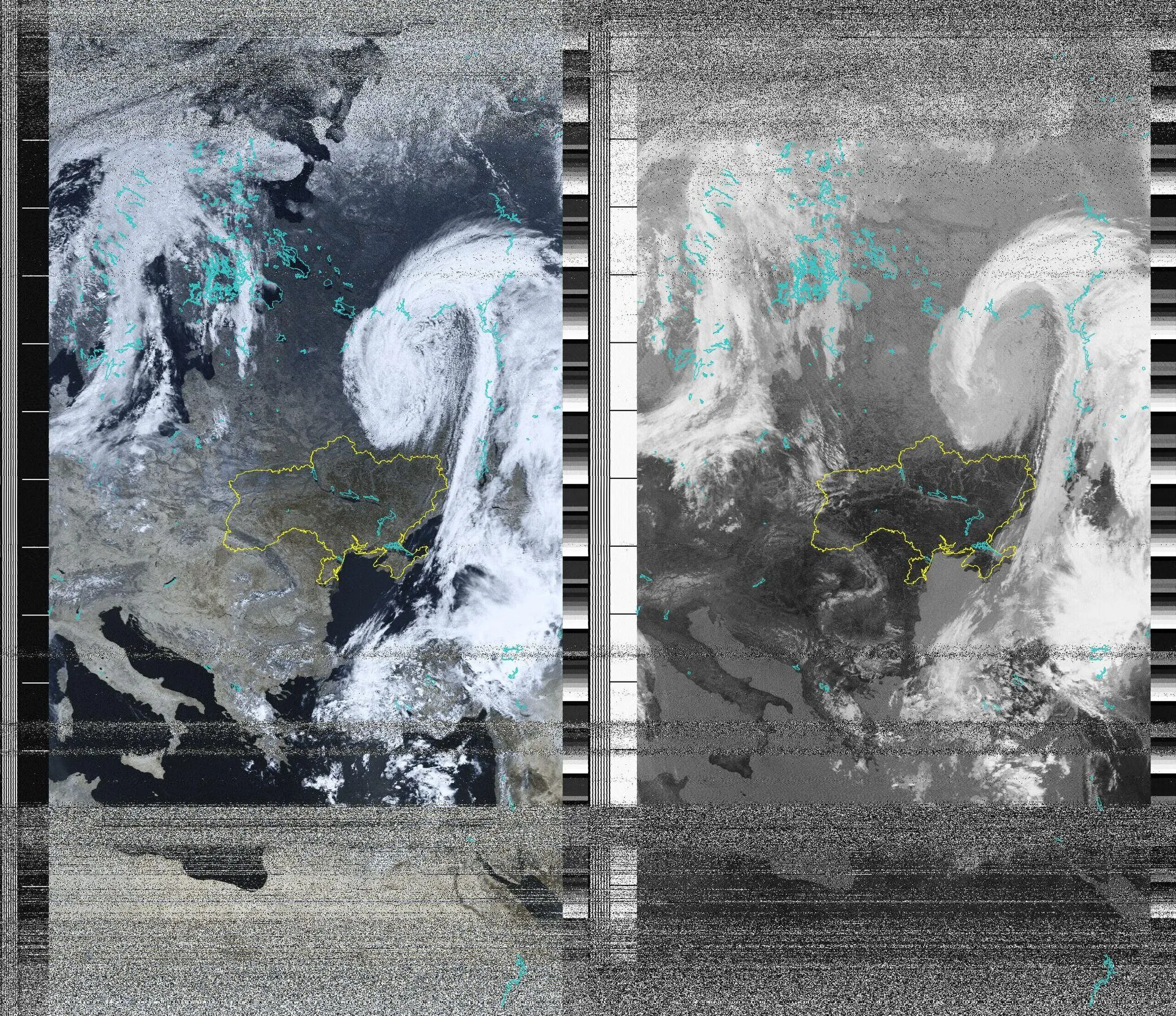
A historical NOAA-19 APT image received directly on 137.100 MHz in May 2025. NOAA APT ended later that year; live weather-satellite work now means digital METEOR-M LRPT instead. NOAA, Wikimedia Commons, public domain.
Listen to the International Space Station
The ISS is a particularly nice target because most people already know what it is, but the word pass needs explaining if you have not tracked satellites before.
The station circles Earth roughly once every 90 minutes, completing about 16 orbits each day. It does not pass over your location every 90 minutes because its orbit is inclined and Earth is rotating underneath it. A pass is simply the period when the ISS is above your local horizon and therefore has a possible line-of-sight radio path to your antenna.
A pass prediction usually gives you AOS, acquisition of signal, when the station rises above your horizon; maximum elevation, the highest angle it reaches above your horizon; and LOS, loss of signal, when it drops below the horizon again. A good high pass may be receivable for roughly eight to ten minutes. Low passes are shorter and harder because buildings, terrain and the longer radio path near the horizon all work against you.
Passes tend to arrive in groups as the orbital ground track moves relative to your location. You may have several useful opportunities over a day or two, then a run of less convenient ones. There is no reason to calculate this by hand.
Pass-prediction tools
This is what I use on iOS. It gives pass times, direction and alerts; the extensions add radio and weather satellites.
A full desktop tracker for satellites, passes, azimuth and elevation.
Enter your position and get upcoming ISS passes without installing anything.
Useful if you also want to see the ISS, but it only highlights passes that are favourable for visual observation.
Before each pass, check ARISS Current Status. The amateur equipment aboard the station changes mode and is sometimes switched off for station operations. The ARISS frequency page lists the standard frequencies.
In June 2026, ARISS listed the Columbus cross-band voice repeater with a 437.800 MHz downlink, while the Zvezda radio was being tested with APRS packet data on 437.825 MHz. Standard ISS amateur frequencies also include 145.800 MHz voice downlink, 145.825 MHz VHF packet and 437.550 MHz SSTV, a mode that sends still pictures as audio tones, when that system is in use. Check ARISS before relying on any of those on a particular day.
For the 437.8 MHz downlink, use the short elements vertically. The theoretical quarter-wavelength is about 17 cm, a little longer than the supplied short elements can reach, so use their maximum length or use the long elements collapsed as far as practical. A simple 70 cm whip will also do useful work.
Try itReceive an ISS repeater pass
Centre the display around 437.800 MHz but leave enough spectrum visible on either side to follow Doppler shift. The signal may arrive several kilohertz above the published frequency while the station is approaching, cross that frequency near closest approach, then continue below it as the ISS recedes.
If the repeater is busy, you will hear amateur stations on the downlink. If packet is active instead, you will hear short digital bursts. During an SSTV event, record the audio and decode the images with suitable SSTV software.
What SSTV reception actually looks like
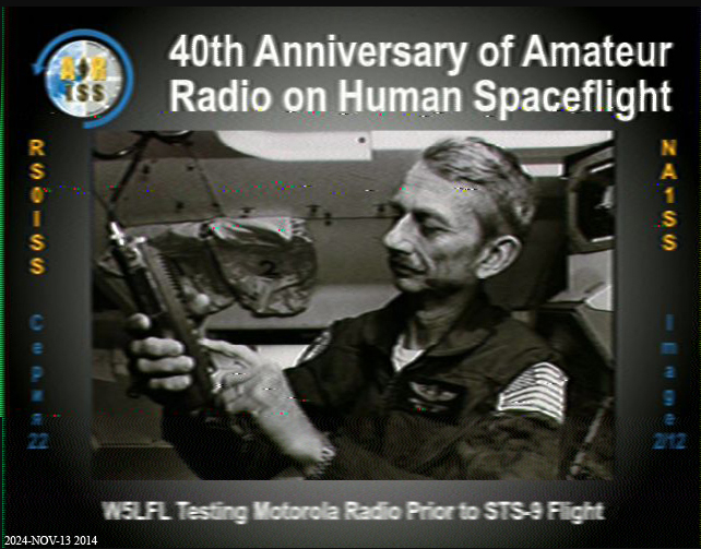
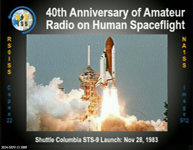
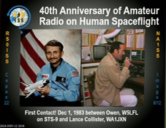
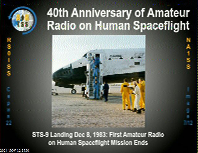
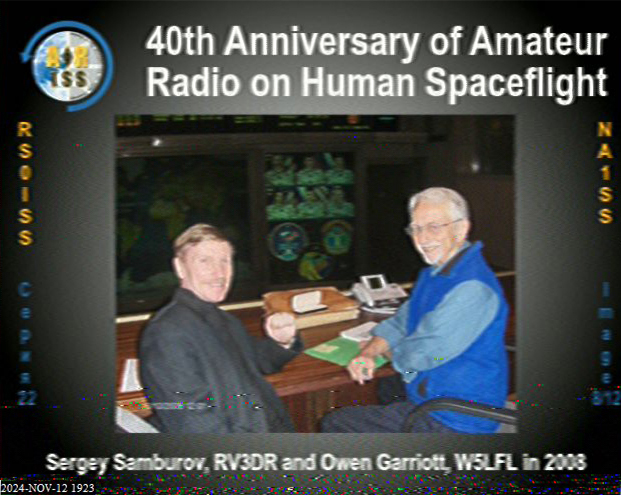
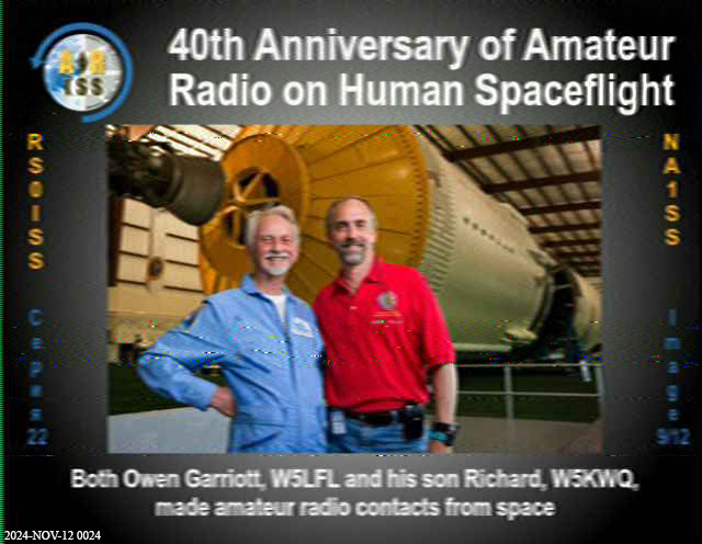
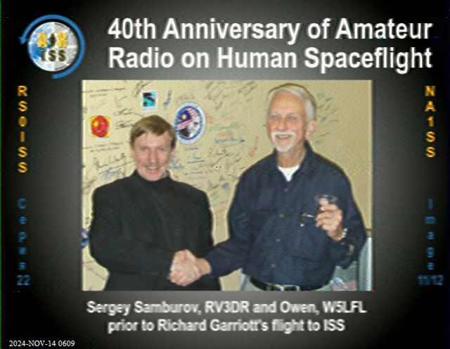
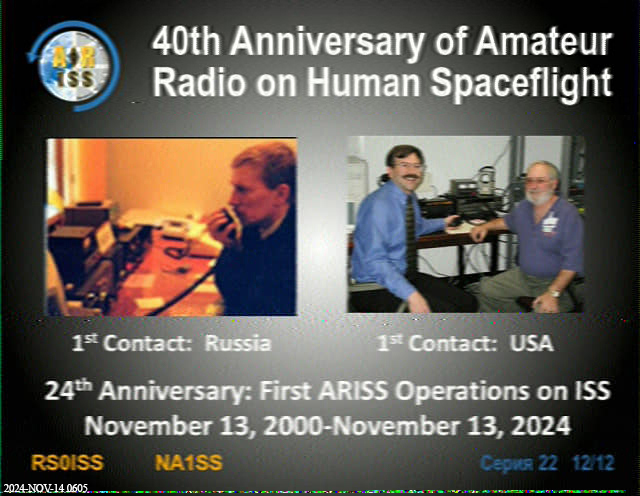
During the November 2024 ARISS SSTV event, I received and decoded nine of the commemorative images transmitted from the International Space Station. They are not pristine downloads, and that is part of what makes them useful. Noise, fading and lost lines remain visible in the finished pictures, so the radio path has left its own record on each one.
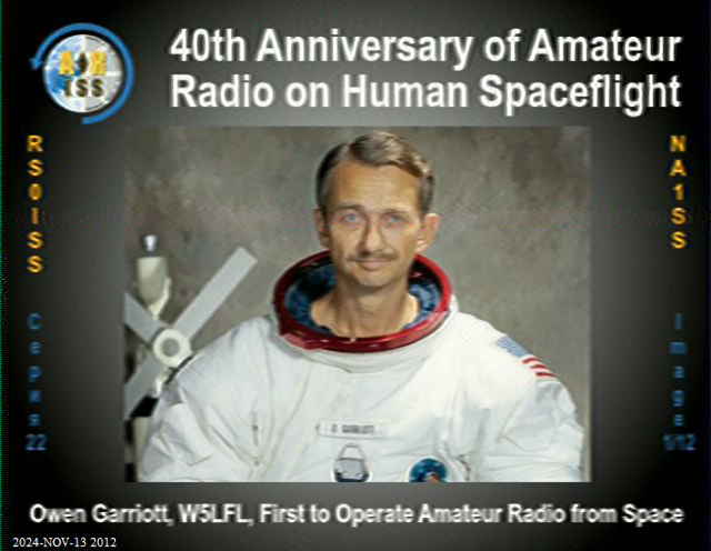


.jpg)
What SSTV sounds like
SSTV sends an image as a sequence of audio tones. This 2 minute 20 second recording was received directly from the ISS using my ID-52. It contains a complete SSTV transmission that suitable decoding software can turn back into an image. Turn the volume down before playing it. The tones are not especially musical.
Download the original WAV recordingThis is the original received audio from the ISS, preserved as a WAV so you can try decoding it yourself.
Pay attention to Doppler
Once you start receiving low-Earth-orbit satellites you will notice Doppler shift everywhere. This is the apparent change in frequency caused by motion between the transmitter and receiver, much like the changing pitch of a passing siren. On an ISS UHF pass the signal begins above its published frequency while the station is approaching. The offset gradually decreases, crosses the published frequency around closest approach, then continues below it as the station recedes.
The effect is smaller at VHF because the size of the Doppler shift scales with frequency. It is therefore much more obvious around 437 MHz than around 145 MHz. This matters with digital satellites as well: if the decoder does not compensate automatically, the signal can shift out of a narrow receive filter as the pass develops.
I would keep the waterfall wide enough during the ISS pass to watch this happen. You can follow the signal manually and see the shift change sign as the station goes from approaching you to moving away.
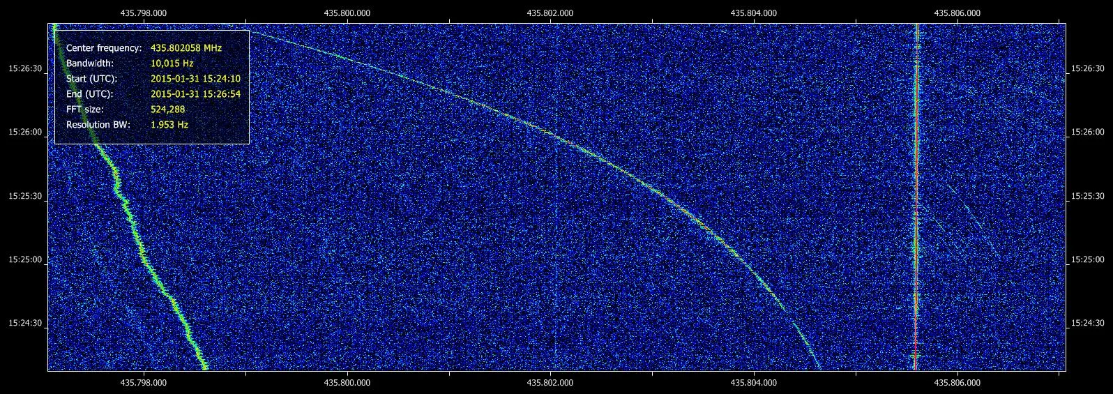
FO-29 received through a satellite pass. The curved traces make the changing Doppler shift visible as the satellite approaches and then recedes. Image: Jan, Hamspirit.
Compare antennas instead of guessing
By now you have already used the supplied antenna in several different configurations. That makes it worth doing a proper comparison rather than deciding one antenna is “better” because the spectrum trace looks taller.
Choose one stable signal. Broadcast FM works well because the transmitter is not moving and is unlikely to stop halfway through the experiment. Set the RF gain and leave it alone. Try a whip, then the dipole at a sensible length. Change the orientation. Put the antenna beside the computer, then use the coax extension to move it to a window. If you can place it outside safely, try that as well.
Watch both the wanted signal and the surrounding noise. Signal strength is commonly shown in decibels (dB). A signal that rises 6 dB while the noise also rises by 6 dB has not bought you much. What matters is the separation between the signal and the noise around it.
Try itWhip versus dipole
Take screenshots if you want to compare later. Keep the centre frequency, gain, spectrum-display scale and filter settings identical between tests.
Find the radio-frequency noise in your house
You can learn quite a lot without receiving anybody else’s transmitter. Radio-frequency noise is unwanted energy from electrical devices that appears in the part of the spectrum you are trying to receive. Find a relatively quiet piece of spectrum and leave the receiver gain unchanged. Put the antenna near a laptop charger, LED lamp, monitor, computer or cheap switch-mode power supply and switch the device on and off.
Some devices will do almost nothing. Others will raise the noise floor, the background level between signals, or produce isolated lines and evenly spaced patterns across the waterfall. This is why radio amateurs can become slightly tedious about power supplies, ferrites, shielding and antenna placement. A surprising amount of radio troubleshooting eventually leads to an innocuous power supply that was never intended to be a transmitter.
Try itHunt for local interference
Try several devices rather than assuming the first charger you pick will be awful. The clean comparison is device off, device on, device off again, with the antenna and receiver left alone.
Start pulling the receiver apart in GNU Radio
Once you are comfortable with the controls in SDR++ or Gqrx, GNU Radio becomes much more useful. Instead of giving you a finished receiver, GNU Radio lets you connect signal-processing blocks to build one yourself. It runs on Windows, macOS and Linux. The GNU Radio installation guide covers the normal routes, while Radioconda provides a convenient cross-platform bundle that includes GNU Radio, Gqrx and related tools.
Go back to FM broadcast because you already know what the result should sound like. A simple GNU Radio Companion receiver can be built as:
If the RTL-SDR is sampling at 2.4 million samples per second (MS/s), one reasonable beginner arrangement is to reduce that stream to 240 thousand samples per second (kS/s) before the FM demodulator, then produce 48 kHz audio for the sound card. GNU Radio calls that rate reduction decimation. The exact values are less important than understanding why each block is there.
The source block chooses the hardware and centre frequency. The filter selects the part of the sampled spectrum you want. The FM demodulator recovers audio from the frequency changes. The audio sink sends the result to the speakers.
Try itRebuild the FM receiver in GNU Radio
Once audio works, add a Frequency Sink or Waterfall Sink before and after the filter. A sink is simply a block that displays or plays the data it receives. Record the raw I/Q samples, the paired numbers used to preserve a radio signal’s amplitude and phase, and play them back later without the dongle connected. That makes the boundary between the physical receiver and the software processing much easier to see.
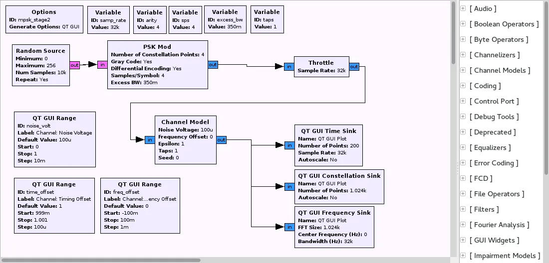
GNU Radio Companion turns the receiver into a visible chain of processing blocks and connections. Screenshot: Bhilburn, Wikimedia Commons, public domain.

For a student who has already worked with Python, data and networks, this is where radio stops looking like a separate hobby. It is another physical source of data that software can sample, filter, interpret and act on.
Amateur radio from here
You can get a surprisingly long way with an RTL-SDR before needing to transmit anything. By this point you may have listened to an amateur repeater, received packets from aircraft, followed an instrument through the atmosphere, received data from orbit, watched Doppler shift on a waterfall, changed an antenna to suit a particular frequency and built part of a receiver in GNU Radio.
That gives the licensing material some context. Frequency allocations, callsigns, modulation modes, antenna design and operating procedures now refer to things you have already encountered rather than things you are being asked to imagine.
In Australia, transmitting on amateur bands requires the appropriate qualification and callsign. The ACMA amateur-radio page explains the current regulatory arrangements, while the WIA Foundation information is a useful starting point for the entry-level qualification.
If this has caught your interest, this is where I would start looking seriously at the Foundation qualification and getting a callsign. The band plan describes frequencies you have already explored, the modulation modes are things you have heard and seen, and antenna dimensions are something you have actually measured.
Then you get to transmit. You can call through a repeater you have been listening to, make simplex contacts, try digital modes, build antennas for both transmit and receive, and eventually communicate directly over the same amateur satellites you started out tracking with the RTL-SDR. The dongle does not become redundant either; it remains a useful second receiver, spectrum display, satellite receiver and general-purpose bit of test gear in an amateur station.
This is VK4MPB saying 73* and going clear on the Chips’nCode repeater.
73 is amateur-radio shorthand for “best regards”.